Conformal Prediction is a relatively new framework for quantifying uncertainities in the predications made by a ML model. It is a method that helps us understand how sure we can be about predictions made by a machine learning model.

Consider, for instance, the multiclass classification task of beans. Utilizing the bean dataset which consists of 8 features describing beans, the objective is to accurately categorize them into one of the 7 varieties: [‘BARBUNYA’, ‘BOMBAY’, ‘CALI’, ‘DERMASON’, ‘HOROZ’, ‘SEKER’, ‘SIRA’].

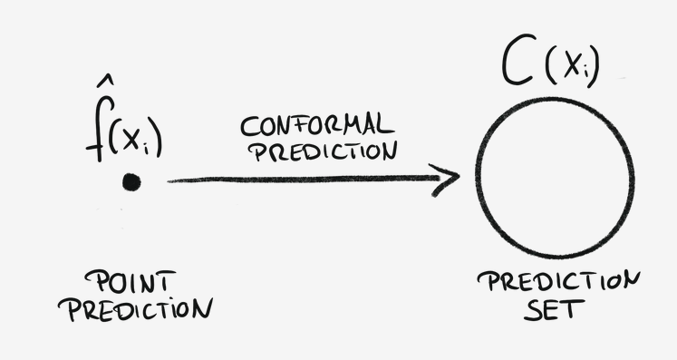
Suppose we’ve employed a classifier model and achieved an accuracy rate of 75%. This means that, on average, out of 100 predictions the model makes, approximately 75 of them are correct. However, accuracy alone doesn’t tell us how confident we can be in each individual prediction. But is there a way to get a set of predictions with different bean varities like [‘BARBUNYA’, ‘CALI’, ‘SIRA’] for which we could say, “We’re 90% sure that the right variety is within this set.”

While classical methods have been employed to address this challenge of Uncertainity Quantification (UQ), they often exhibit limitations and drawbacks. Conformal Prediction provides us with precisely this capability. It allows us to generate prediction sets with specified confidence levels. In this article, using Conformal Prediction, implementation we can obtain a set of predictions for each bean instance, ensuring that with, say, 90% confidence, the correct bean type lies within that set.

Traditional Methods for UQPermalink

1. Bootstrapping : Bootstrapping involves generating multiple bootstrap samples from the dataset and observing variations in the model’s predictions across these samples. This approach provides insight into the variability of predictions but can be computationally expensive.

2. Ensemble Methods: Ensemble methods aggregate predictions from multiple base models to measure variability or spread in predictions. While these methods can provide a sense of uncertainty, they come with limitations:
   • Models need to be trained multiple times, increasing computational costs.
   • Probabilities generated by ensemble methods (e.g., Random Forests) may resemble uncertainty scores but are often not well-calibrated.

   Probabilities are considered calibrated when their predicted confidence matches the observed accuracy. For instance, if a model predicts a class with 80% confidence, it should be correct 8 out of 10 times for that class.

3. Bayesian Networks : Bayesian networks explicitly model uncertainty through probability distributions. They update beliefs about parameters using Bayesian inference, deriving uncertainty measures from the resulting posterior distributions.
   However, this method has challenges:
   • Incorporating robust uncertainty into the prior distributions requires careful consideration.
   • Bayesian approaches often rely on strong distributional assumptions and may not always produce well-calibrated uncertainty estimates.

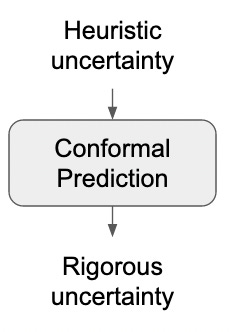
Conformal Prediction overcomes these shortcomings and it is very simple to implement. Conformal Prediction is a versatile method that can turn any uncertainity measure into a rigorous one.

Instructions for Conformal PredictionPermalink

Step 1: Training

• Divide the dataset into training, calibration, and test sets.
• Train the machine learning model using the training data.

Step 2: Calibration

• Use a pre-trained model $\hat{f}$ to determine a heuristic representation of uncertainty. This can often be achieved using probability estimates obtained from model.predict_proba().
• Define a score function $s(X,y)$ where larger scores indicate poorer agreement between input features $X$ and true labels $y$. A simple option is to use $1 -$ model.predict_proba().
• Calculate scores on the calibration data of size $n$.
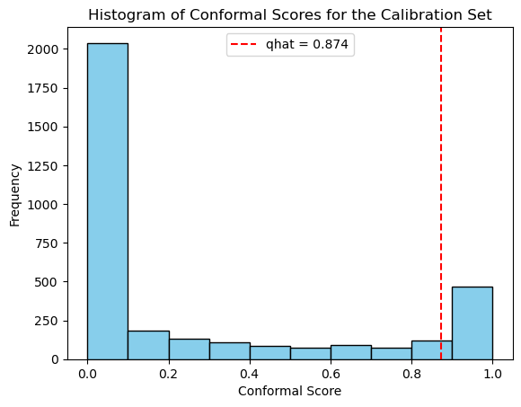
• Compute $\hat{q}$ as the $\frac{(⌈(𝑛+1)(1−𝛼)⌉)}{𝑛}$ quantile of the calibrated scores, where $\alpha$ represents the desired error rate.

Step 3: Prediction

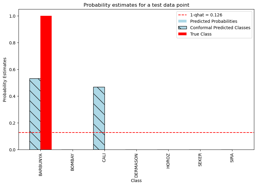
• Utilize the quantile to construct prediction sets for new data in the test set. $C(X_{\text{test}}) = \left \{ y : s(X_{\text{test}}, y) \leq \hat{q} \right \}$

• Ensure that the probability of the true output lying within the prediction set is at least $1 - \alpha$. $𝑃(y_{\text{test}} \in C(X_{\text{test}})) \geq 1-\alpha$.

  1−𝛼 Coverage Guarantee: This guarantees that the true output has a probability of at least $(1-\alpha)$ to be included in the prediction set.

Split Conformal Prediction: Beans ClassificationPermalink

# Step 1: Training
model = GaussianNB().fit(X_train, y_train)

# Step 2: Calibration
y_cal_predictions = model.predict_proba(X_cal)
prob_true_class = y_cal_predictions[np.arange(len(y_cal)), y_cal]
q_level = np.ceil((n + 1)*(1 - alpha))/n
qhat = np.quantile(1  -prob_true_class, q_level) 

# Step 3: Predictions
y_test_predictions = model.predict_proba(X_test)
predictions_set = (1 - y_test_predictions <= qhat)

The Gaussian Naive Bayes model was used to train a dataset.

We are $87.4\%$ certain that the true variety of the bean is BARBUNYA.

AdvantagesPermalink

• Guaranteed Coverage: Conformal prediction ensures that the true output lies within the prediction set with a specified confidence level, providing a strong and reliable coverage guarantee.

• Model-Agnostic: This approach works seamlessly with any machine learning model. It can take any heuristic notion of uncertainty from a model and transform it into a rigorous, interpretable prediction set.

• Distribution-Free: Conformal prediction makes less assumptions about the underlying distributions of the data. It only requires that the calibration set and the test set are independent and identically distributed (i.i.d.) and exchangeable.

• Ease of Implementation: The framework is simple to implement and can be applied to a wide variety of problems, making it a versatile tool for uncertainty quantification.

Extensions of Conformal PredictionPermalink

1. Different Choices of Score Function: Conformal prediction allows flexibility in defining score functions, enabling tailored approaches to uncertainty quantification for different tasks or datasets.

2. Conformal Risk Control:
   For any bounded loss function $l$, which decreases as the prediction set $C$ grows, conformal prediction provides guarantees on the expected risk. Specifically, it ensures that:

   $$\mathbb{E}[l(C_\lambda(X_{\text{test}}), y_{\text{test}})] \leq \alpha$$

   This means the risk of incorrect predictions, as measured by the chosen loss function, remains below the desired threshold $\alpha$. This extension is particularly useful in scenarios where it’s important to balance coverage with the cost of overly large prediction sets.

3. Adaptive Prediction Sets: By dynamically adjusting prediction sets based on input features, adaptive prediction sets aim to optimize their size while preserving the desired confidence level.

4. Conformalized Quantile Regression: This method extends conformal prediction to regression tasks, allowing the construction of prediction intervals that adapt to the variability in the data.

ReferencesPermalink

1. Course On Conformal Prediction: Christoph Molnar
2. Awesome conformal prediction
3. A gentle introduction to conformal prediction. Angelopoulos and Bates, 2022