Corporate Credit Rating Forecast using Machine Learning Methods

Introduction

Corporate credit ratings, issued by credit rating agencies like Standard & Poor’s and Moody’s, express the agency’s opinion about the ability of a company to meet its debt obligations. Typically, ratings are expressed as letter grades that range, for example, from ‘AAA’ to ‘D’ to communicate the agency’s opinion of relative level of credit risk. Credit ratings are not absolute measures of Default Probability. For example, a corporate bond that is rated ‘AA’ is viewed by the rating agency as having a higher credit quality than a corporate bond with a ‘BBB’ rating. But the ‘AA’ rating isn’t a guarantee that it will not default, only that, in the agency’s opinion, it is less likely to default than the ‘BBB’ bond.

Investors and other market participants may use these ratings as a screening device to match the relative credit risk of an issuer or individual debt issue with their own risk tolerance or credit risk guidelines in making investment and business decisions. For instance, in considering the purchase of a corporate bond, an investor may check to see whether the bond’s credit rating aligns with their acceptable level of credit risk. At the same time, credit ratings may be used by corporations to help them raise money for expansion and/or research and development.

Each credit rating agency applies its own methodology to measure creditworthiness and this assessment is an expensive and complicated process. Usually, the agencies take time to provide new ratings and update older ones. This causes delays in decision-making process for the investors.

One solution to address these delays would be to use the historical financial information of a company to build a predictive quantitative model capable of forecasting the credit rating that a company will receive. In this project, machine learning techniques have been utilized to create classification models capable of rapidly forecasting credit ratings. Machine learning stands out in this context due to its adaptability and ability to capture complex patterns in data, providing a more dynamic and responsive approach compared to traditional quantitative models.

Dataset

The Corporate Credit Rating dataset was obtained from Kaggle. The dataset loaded as a pandas dataframe, ratings_df, consists of 2029 entries (rows) and 31 columns. Each entry represents a big US firm traded on NYSE or Nasdaq. The ratings span the period from 2010 to 2016. The dataset has 593 unique US firms, as seen from ratings_df.Name.value_counts().

Credit Ratings

The target variable is the Rating column, representing the credit rating assigned by agencies. Taking a closer look at the list of agencies and their different ratings using ratings_df['Rating Agency Name'].value_counts() and ratings_df.groupby('Rating Agency Name')['Rating'].unique():

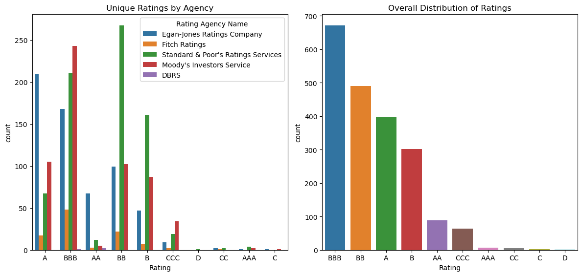
The dataset shows an imbalance in credit ratings, with varying frequencies for each rating category as it is evident from ratings_df.Rating.value_counts().

An additional challenge is that we have ratings from different agencies. This was addressed by simplifying and merging the ratings labels according to the following table from Investopedia: Corporate Credit Ratings

Moody’s	Standard & Poor’s	Fitch	Grade	Risk
Aaa	AAA	AAA	Investment	Lowest Risk
Aa	AA	AA	Investment	Low Risk
A	A	A	Investment	Low Risk
Baa	BBB	BBB	Investment	Medium Risk
Ba, B	BB, B	BB, B	Junk	High Risk
Caa/Ca	CCC/CC/C	CCC/CC/C	Junk	Highest Risk
C	D	D	Junk	In Default

A dictionary was used for the mapping of new ratings and old ratings and ratings_df['Rating'].map(rating_dict) and we have regrouped the 10 different rating categories into 6 new categories.

(New) Rating	Counts	(Old) Ratings
‘Lowest Risk’	7	‘AAA’
‘Low Risk’	487	‘AA’, ‘A
‘Medium Risk’	671	‘BBB’
‘High Risk’	792	‘BB’, ‘B’
‘Highest Risk’	71	‘CCC’ ‘CC’, ‘C’
‘In Default’	1	‘D’

The rows with the Ratings: 'Lowest Risk and 'In Default are dropped from the dataset given their small value counts.

The categorical variable Rating was converted into numerical labels using the LabelEncoder from scikit-learn’s preprocessing module, assigning a distinct integer code to each unique label.

Input Features

The other columns in the dataset are the input features related to financial indicators and information about the company.

The 5 features with the company information such as Name, Symbol (for trading), Rating Agency Name, Date, and Sector provide context and additional details for analysis but their inclusion in the model may not be necessary for the specific task of credit rating prediction. However, the Sector feature has been included in our model as it is crucial for capturing industry-specific nuances that significantly influence a company’s financial performance and risk profile.

In order to integrate the categorical data Sector into the model, LabelEncoder was employed to represent it numerically.

The dataset includes 25 financial indicators that can be categorized into different groups. These financial indicators collectively provide a comprehensive view of a company’s financial health and performance, contributing to the evaluation of its creditworthiness.

(I) Liquidity Measurement Ratios These ratios provide insights into a company’s short-term financial health and ability to meet its immediate obligations.

1. currentRatio: Indicates the company’s ability to cover short-term liabilities with short-term assets.
2. quickRatio: Measures the company’s ability to cover immediate liabilities without relying on inventory.
3. cashRatio: Reflects the proportion of cash and cash equivalents to current liabilities.
4. daysOfSalesOutstanding: Measures the average number of days it takes for a company to collect payment after a sale.

(II) Profitability Indicator Ratios These ratios evaluate a company’s ability to generate profits relative to its revenue and investments.

1. netProfitMargin: Represents the percentage of profit relative to total revenue.
2. pretaxProfitMargin: Measures profitability before taxes are considered.
3. grossProfitMargin: Indicates the percentage of revenue retained after deducting the cost of goods sold.
4. operatingProfitMargin: Reflects the company’s profitability from its core operations.
5. returnOnAssets: Gauges how efficiently a company utilizes its assets to generate earnings.
6. returnOnEquity: Measures the return generated on shareholders’ equity.
7. returnOnCapitalEmployed: Assesses the efficiency of capital utilization in generating profits.
8. ebitPerRevenue: Measures earnings before interest and taxes relative to revenue.

(III) Debt Ratios These ratios assess the company’s leverage and debt management.

1. debtEquityRatio: Measures the proportion of debt relative to equity.
2. debtRatio : Represents the percentage of a company’s assets financed by debt.

(IV) Operating Performance Ratios These ratios focus on operational efficiency and effectiveness.

1. assetTurnover: Evaluates how efficiently a company utilizes its assets to generate sales revenue.
2. fixedAssetTurnover : Measures the efficiency of generating sales from fixed assets.
3. payablesTurnover: Measures the efficiency of a company’s payment of its liabilities.

(V) Cash Flow Indicator Ratios These ratios delve into a company’s cash flow dynamics, providing insights into its financial sustainability.

1. operatingCashFlowPerShare: Reflects the cash generated by core business operations per share.
2. freeCashFlowPerShare: Measures the amount of cash available to shareholders after covering operational expenses and capital expenditures.
3. cashPerShare: Represents the amount of cash available per outstanding share.
4. operatingCashFlowSalesRatio: Evaluates the percentage of sales revenue converted into cash from operating activities.
5. freeCashFlowOperatingCashFlowRatio: Measures the efficiency of converting operating cash flow into free cash flow.
6. effectiveTaxRate: Reflects the company’s tax efficiency.
7. companyEquityMultiplier: Indicates the multiplier effect on equity due to debt
8. enterpriseValueMultiple: Evaluates a company’s overall value relative to its earnings.

Descriptive Statistics

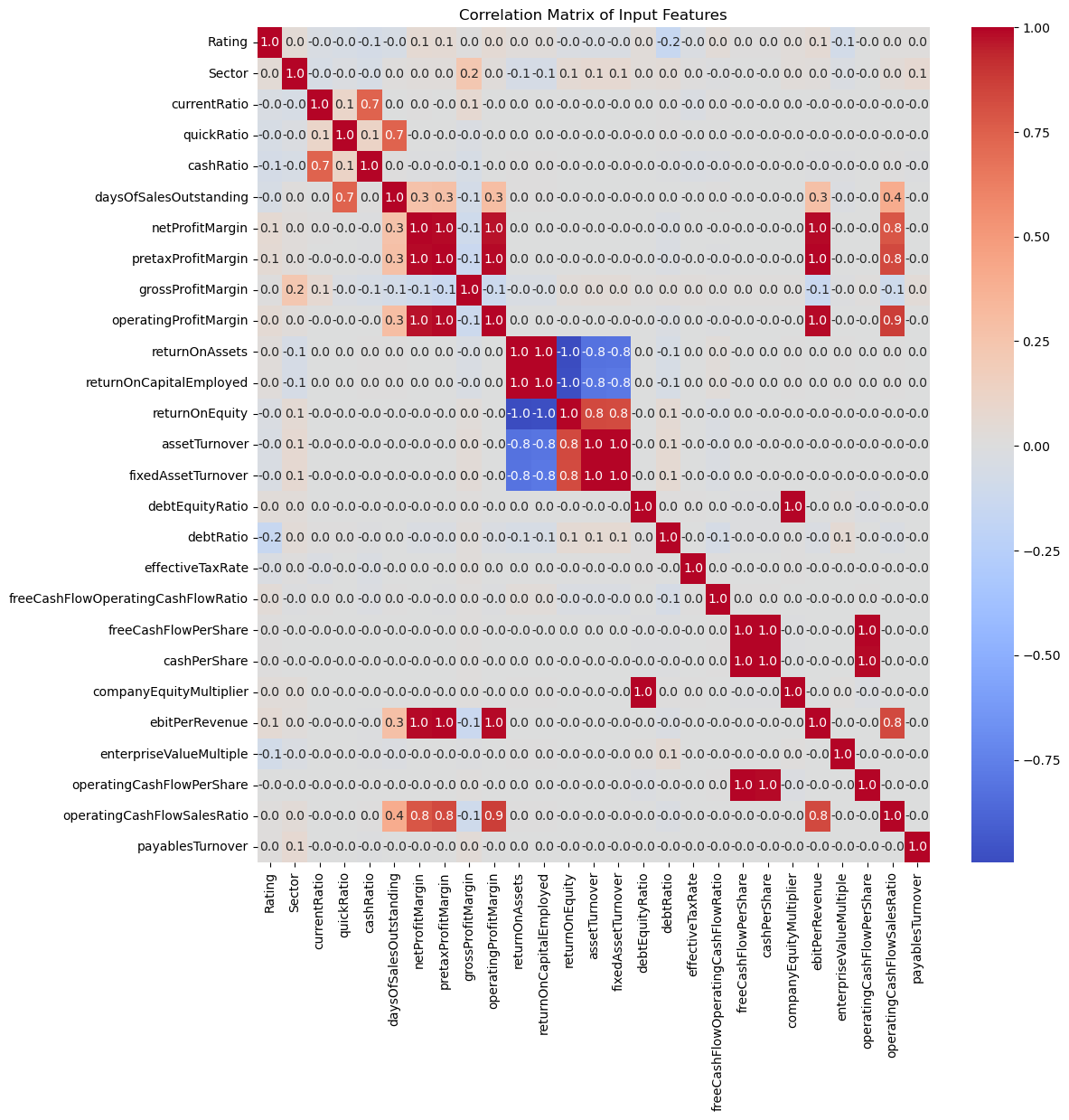
The correlation matrix ratings_df.corr() was calculated to understand the pairwise correlations between different variables in the dataset. A correlation value close to 1 indicates a strong positive correlation, while a value close to -1 indicates a strong negative correlation. From the figure below, it is seen that the target Rating has low correlation with almost all of the input features. It is also observed that companies with higher Return on Equity tend to also have higher Asset Turnover and Fixed Asset Turnover, indicating that they efficiently use their assets, both overall and fixed assets, to generate profits.

The describe() function was used to understand the statistical descriptions like mean, min, max, percentiles of the numerical financial indicators. Comparison of the mean to the median and examining the range between percentiles indicated the presence of outliers.

Features also exhibit different scales, as evident from the magnitude of mean and standard deviation values. Feature scaling was performed to ensure equal contribution from all features for machine learning algorithms. The Min-Max scaling technique was applied to normalize the numerical values representing financial indicators.

\[x_{scaled} = \frac{x - x_{min}}{x_{max} - x_{min}}\]

For each column, the MinMaxScaler function from sklearn.preprocessing was used to transform the values into a standardized range between 0 and 1. The values are then multiplied by 1000, to amplify the scaled values.

Additionally, a logarithmic transformation was applied to each value using the np.log10 function, with a small constant (0.01) added to avoid issues with zero values. This dual transformation approach normalizes and potentially enhance the interpretability of the financial indicators in the dataset.

This work in exploring and preparing our dataset, sets the stage for the next phase: deploying different machine learning models to forecast credit ratings.

ML Models and Training

Our problem of corporate credit rating forecast is a supervised multi-class classification task.

The input data was divided into training and testing sets, using the train_test_split() function from sklearn.model_selection. This function randomly separates the data into two subsets, ensuring that both subsets maintain the distribution of the target variable. The training set, comprising 80% of the data, was used for model training, while the remaining 20% formed the test set for model evaluation. The input features (X) and target lables (y) are then identified in each set and assigned to separate dataframes.

The following machine learning models were employed to forecast corporate credit ratings.

1. Logistic Regression: Logistic Regression is a linear model used for binary or multiclass classification. It estimates the probability that a given instance belongs to a particular class. It employs the logistic function (sigmoid) to transform a linear combination of input features into a value between 0 and 1. This output represents the probability of belonging to the positive class. A threshold is applied to make the final classification decision.

2. K-Nearest Neighbors (KNN): KNN is a non-parametric algorithm used for classification. It classifies a data point based on the majority class among its k-nearest neighbors. The algorithm calculates the distance between the input instance and all data points in the training set. It then assigns the class that is most common among the k-nearest neighbors.

3. Support Vector Machine (SVM): SVM is a powerful classification algorithm that aims to find a hyperplane in a high-dimensional space that best separates data points of different classes. SVM transforms input features into a higher-dimensional space and seeks a hyperplane that maximizes the margin between classes. It classifies instances based on which side of the hyperplane they fall on.

4. Random Forest: Random Forest is an ensemble learning method that constructs a multitude of decision trees during training and outputs the mode of the classes for classification tasks. It builds multiple decision trees using a subset of features and a random subset of the training data. The final prediction is determined by aggregating the predictions of individual trees (voting or averaging).

5. Gradient Boost: Gradient Boosting is an ensemble learning method that builds a series of weak learners (typically decision trees) sequentially, each correcting the errors of its predecessor. It fits a weak model to the residuals of the previous model. This process continues, with each new model focusing on the mistakes of the ensemble. The final prediction is a weighted sum of the predictions from all weak models.

6. XGBoost: XGBoost (Extreme Gradient Boosting) is an advanced version of gradient boosting that incorporates regularization and parallel processing, making it highly efficient. Similar to gradient boosting, XGBoost builds a series of trees sequentially. It optimizes a regularized objective function, combining the prediction from each tree. It uses a technique called boosting to strengthen the model iteratively.

The models were import from their respective standard libraries and initialized with their specific parameters. The models were trained on the training dataset (X_train, y_train) using the .fit() method and evaluated on the test dataset (X_test, y_test) using .predict(). The accuracy of each model was calculated using the metrics.accuracy_score function from scikit-learn.

models = {
    'Logistic Regression': LogisticRegression(random_state=2996 , multi_class='multinomial', solver='newton-cg'),
    'K-Nearest Neighbors': KNeighborsClassifier(n_neighbors = 4),
    'Support Vector Machine': svm.SVC(kernel='rbf', gamma= 1.5, C = 4, random_state=2996),
    'Random Forest':  RandomForestClassifier(random_state=2996),
    'Gradient Boost': GradientBoostingClassifier(random_state=2996),
    'XGBoost': xgb.XGBClassifier(objective ='multi:softmax', num_class=4),
}

predictions = []
accuracies = []

for model_name, model in models.items():
    model.fit(X_train, y_train)
    y_pred = model.predict(X_test)
    accuracy = metrics.accuracy_score(y_test, y_pred)
    
    predictions.append((model_name, y_pred))
    accuracies.append((model_name, accuracy))
    print(f"{model_name} Accuracy: {accuracy}")

SMOTE

The Synthetic Minority Over-sampling Technique (SMOTE) was applied in an attempt to address the issue of class imbalance observed in the training dataset, as indicated by y_train.value_counts(). This imbalance could potentially introduce bias in the model predictions. The SMOTE algorithm, implemented through the SMOTE function from the imblearn.over_sampling library, was utilized to create synthetic instances of the minority class, effectively balancing the distribution of ratings.

Following this, the models were trained with the resampled dataset (X_train_resampled, y_train_resampled) and evaluated on the(X_test, y_test).

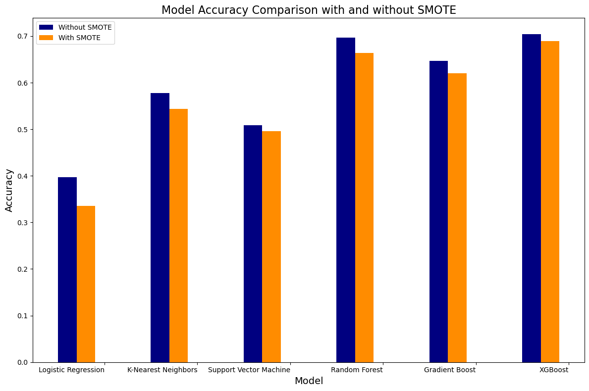
It was observed that the accuracy slightly decreased after employing SMOTE. This phenomenon could be attributed to the introduction of synthetic samples, potentially leading to increased noise and complexity in the dataset. Moreover, the choice of sampling strategy in SMOTE, 'auto', might have not been optimal for our problem. Alternative methods, including undersampling or experimenting with different SMOTE sampling strategies, could be considered. For the current scope of the project, SMOTE resampling has been omitted.

Hyperparameter Optimisation

Hyperparameter optimization was performed for the XGBoost model.

RandomizedSearchCV is a method for hyperparameter tuning that explores a defined number of random combinations of hyperparameters. A parameter grid xgb_params was defined with XGBoost hyperparameters such as learning rate, number of estimators, maximum depth, minimum child weight, subsample, and colsample by tree. The n_iter was set to 15 and the search was performed through 15 different combinations. The StratifiedKFold was employed for cross-validation. It ensures that each fold preserves the same distribution of target classes as the entire dataset, which is crucial for maintaining the representation of different credit ratings in each fold.

The metric used for evaluation was accuracy (scoring='accuracy'). The search was parallelized (n_jobs=-1), making use of all available CPU cores. The model was fitted to the training data to identify the best hyperparameters. The best model with optimal hyperparameters was then extracted from the search results. Finally, the best model was evaluated on the test set, and the accuracy was noted.

xgb_params = {
        'learning_rate': [0.01, 0.1, 0.2],
        'n_estimators': [100, 200, 300],
        'max_depth': [3, 5, 7],
        'min_child_weight': [1, 3, 5],
        'subsample': [0.8, 0.9, 1.0],
        'colsample_bytree': [0.8, 0.9, 1.0]
    },
 
# Create StratifiedKFold for cross-validation
cv = StratifiedKFold(n_splits=5, shuffle=True, random_state=2996)

# Create RandomizedSearchCV
random_search = RandomizedSearchCV(
    estimator= xgb.XGBClassifier(objective ='multi:softmax', num_class=4),
    param_distributions=xgb_params,
    n_iter=15,  
    scoring='accuracy',
    n_jobs=-1,
    cv=cv,
    random_state=2996
)

# Fit the model to find the best hyperparameters
random_search.fit(X_train, y_train)

# Get the best model with optimal hyperparameters
best_model = random_search.best_estimator_

# Evaluate the model on the test set
best_y_pred = best_model.predict(X_test)
best_accuracy = metrics.accuracy_score(y_test, best_y_pred)

The accuracy after hyperparameter optimisation for the XGBoost 0.69, was found to be very close to the initial model accuracy of 0.70.

Results

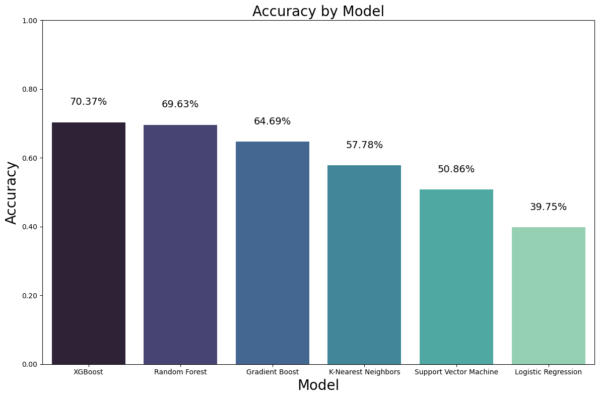
XGBoost and Random Forest exhibited the highest accuracies, with Gradient Boosting closely following. On the other hand, Logistic Regression showed comparatively lower performance in terms of accuracy.

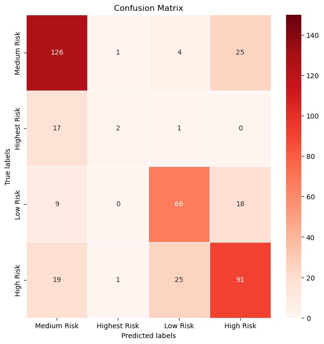
The distribution of true positive, true negative, false positive, and false negative predictions were observed from the confusion_matrix.

A summary of key classification metrics, including accuracy, precision, recall, and F1 score was obtained using classification_report from sklearn.metrics

• Accuracy reflects the overall correctness of the model’s predictions.

  \(\frac{TP + TN}{TP + TN + FP + FN}\) where

  True Positive (TP): The number of instances correctly predicted as positive.
  True Negative (TN): The number of instances correctly predicted as negative.
  False Positive (FP): The number of instances wrongly predicted as positive (Type I error).
  False Negative (FN): The number of instances wrongly predicted as negative (Type II error).

• Precision measures the proportion of true positive predictions among instances predicted as positive, highlighting the model’s ability to avoid false positives. High precision indicates a low rate of false positives. \(\frac{TP}{TP + FP}\)
• Recall gauges the model’s effectiveness in capturing true positives among all actual positive instances. High recall indicates a low rate of false negatives. \(\frac{TP}{TP + FN}\)
• F1 score is the harmonic mean of precision and recall, providing a single metric that considers both false positives and false negatives. F1-score values range from 0 to 1, and higher values indicate better balance between precision and recall.

Each row in the classification report corresponds to a specific class, and the support column indicates how many instances in the dataset belong to that class. The overall performance is best on the Medium Risk Class and worst on the Highest Risk Class, and this could be related to the imbalance in the input dataset.

Class	precision	recall	f1-score	support
Medium Risk	0.74	0.81	0.77	156
Highest Risk	0.50	0.10	0.17	20
Low Risk	0.69	0.71	0.70	93
High Risk	0.68	0.67	0.67	136

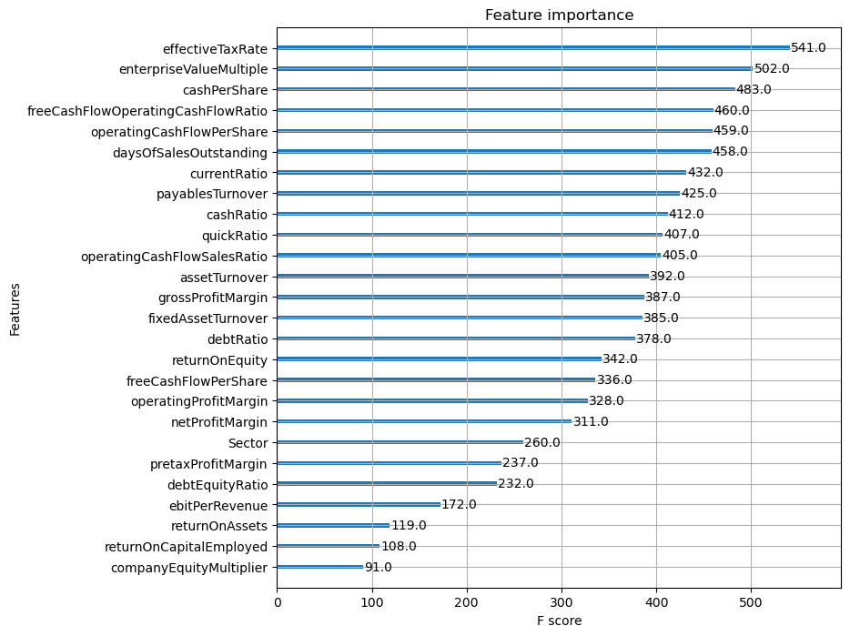
The contribution of each input feature to the XGBoost model’s decision-making process is visualized through the feature importance plot. This helps in understanding which financial indicators play a significant role in predicting credit ratings.

It was observed that the features Effective Tax Rate, Enterprise Value Multiple, Cash per Share might have a stronger relationship with credit ratings. And the financial indicators Company Equity Multiplier, Return on Capital Employed, Return on Assets might have less impact on predicting credit ratings in this dataset.

Applications

The classification methods implemented in this project can be extended to predict Environmental, Social, and Governance (ESG) Ratings that assess a company’s performance and behavior in key areas related to sustainability and ethical practices. ESG ratings are primarily used by investors to evaluate the sustainability of a company’s business model and assess its long-term objectives.

These classification algorithms are equally valuable for analyzing historical stock data. By predicting whether a stock price will increase, decrease, or remain stable, investors gain valuable insights to make well-informed decisions in the dynamic stock market environment.

References

1. Parisa Golbayani, Ionuţ Florescu, Rupak Chatterjee: A comparative study of forecasting corporate credit ratings using neural networks, support vector machines, and decision trees. The North American Journal of Economics and Finance, Volume 54, 2020, DOI

2. Kaggle Datasets: Corporate Credit Rating

3. S&P Global: Guide to Credit Rating Essentials